ANN Benchmark

This vector database benchmark is designed to measure and illustrate Weaviate's Approximate Nearest Neighbor (ANN) performance for a range of real-life use cases.

To make the most of this vector database benchmark, you can look at it from different perspectives:

The overall performance – Review the benchmark results to draw conclusions about what to expect from Weaviate in a production setting.
Expectation for your use case – Find the dataset closest to your production use case, and estimate Weaviate's expected performance for your use case.
Fine Tuning – If you don't get the results you expect. Find the optimal combinations of the configuration parameters (efConstruction, maxConnections and ef) to achieve the best results for your production configuration. (See HNSW Configuration Tips)

Measured Metrics

For each benchmark test, we set these HNSW parameters:

efConstruction - Controls the search quality at build time.
maxConnections - The number of outgoing edges a node can have in the HNSW graph.
ef - Controls the search quality at query time.

For each set of parameters, we've run 10,000 requests, and we measured the following metrics:

The Recall@10 and Recall@100 - by comparing Weaviate's results to the ground truths specified in each dataset.
Multi-threaded Queries per Second (QPS) - The overall throughput you can achieve with each configuration.
Individual Request Latency (mean) - The mean latency over all 10,000 requests.
P99 Latency - 99% of all requests (9,900 out of 10,000) have a latency that is lower than or equal to this number
Import time - Since varying build parameters has an effect on import time, the import time is also included.

By request, we mean: An unfiltered vector search across the entire dataset for the given test. All latency and throughput results represent the end-to-end time that your users would also experience. In particular, these means:

Each request time includes the network overhead for sending the results over the wire. In the test setup, the client and server machines were located in the same VPC.
Each request includes retrieving all the matched objects from disk. This is a significant difference from ann-benchmarks, where the embedded libraries only return the matched IDs.

Benchmark Results

This section contains datasets modeled after the ANN Benchmarks. Pick a dataset that is closest to your production workload:

Dataset	Number of Objects	Vector Dimensions	Distance metric	Use case
SIFT1M	1 M	128	l2-squared	SIFT is a common ANN test dataset generated from image data
DBPedia OpenAI	1 M	1536	cosine	DBPedia dataset from MTEB embedded with OpenAI's ada002 model
MSMARCO Snowflake	8.8 M	768	l2-squared	MSMARCO dataset embedded with Snowflake's Arctic Embed M v1.5 model
Sphere DPR	10 M	768	dot	Meta's Sphere dataset (10M sample)

Benchmark Datasets

These are the results for each dataset:

QPS vs Recall for DBPedia OpenAI

DBPedia OpenAI Benchmark results

efConstruction	maxConnections	ef	Recall	QPS	Mean Latency	p99 Latency	Import Time
256	16	16	84.32	12183	1.29	2.14	286
128	16	16	83.28	11927	1.32	2.24	168
384	16	16	84.69	11843	1.32	2.26	401
256	16	24	89	10816	1.46	2.42	286
128	16	24	88.08	10540	1.5	2.56	168
384	16	24	89.18	10486	1.5	2.65	401
128	32	16	88.55	10426	1.51	2.67	216
256	32	16	89.72	9801	1.6	2.65	439
256	16	32	91.56	9563	1.65	2.83	286
128	32	24	92.25	9167	1.72	2.89	216
384	16	32	91.74	8902	1.77	4.21	401
128	16	32	90.65	8796	1.79	4.06	168
384	32	16	89.92	8734	1.81	5.44	620
256	32	24	93.42	8024	1.97	4.07	439
128	32	32	94.26	8011	1.97	3.34	216
384	16	48	94.49	7912	1.99	3.3	401
384	32	24	93.64	7894	1.99	3.23	620
256	16	48	94.36	7831	2.02	3.95	286
256	32	32	95.18	7434	2.12	3.58	439
128	16	48	93.57	7279	2.17	4.97	168
128	16	64	95.02	7061	2.23	3.63	168
256	16	64	95.75	7004	2.26	3.77	286
384	32	32	95.46	6910	2.28	3.76	620
384	16	64	95.94	6907	2.28	3.81	401
128	32	48	96.24	6613	2.38	4.14	216
256	32	48	97.07	6072	2.59	4.3	439
128	16	96	96.51	5672	2.77	4.51	168
256	16	96	97.24	5639	2.8	4.43	286
384	32	48	97.34	5577	2.82	4.51	620
384	16	96	97.4	5457	2.89	4.73	401
128	32	64	97.14	5277	2.98	5.73	216
256	32	64	97.96	5141	3.07	5.04	439
128	16	128	97.32	4794	3.3	5.16	168
256	16	128	97.97	4720	3.35	5.34	286
384	32	64	98.14	4557	3.47	6.61	620
384	16	128	98.14	4482	3.51	5.96	401
128	32	96	98.04	4464	3.51	5.7	216
256	32	96	98.69	4034	3.91	6.19	439
128	32	128	98.51	3749	4.2	6.84	216
384	32	96	98.9	3622	4.34	6.72	620
256	32	128	99.04	3260	4.83	7.89	439
384	32	128	99.25	3011	5.22	7.94	620
128	16	256	98.43	2964	5.3	8.52	168
256	16	256	98.93	2957	5.33	8	286
384	16	256	99.07	2871	5.49	8.12	401
128	32	256	99.15	2334	6.73	11	216
128	16	384	98.85	2279	6.94	10.55	168
256	16	384	99.26	2185	7.25	11.32	286
384	16	384	99.36	2157	7.32	10.8	401
256	32	256	99.56	2013	7.84	12.29	439
384	32	256	99.69	1856	8.53	12.78	620
128	16	512	99.08	1845	8.56	13.06	168
256	16	512	99.42	1783	8.87	13.09	286
384	16	512	99.52	1739	9.12	13.7	401
128	32	384	99.39	1725	9.15	15.57	216
256	32	384	99.73	1517	10.42	16.34	439
128	32	512	99.53	1392	11.31	18.65	216
384	32	384	99.81	1363	11.61	18.18	620
256	32	512	99.81	1220	12.93	20.23	439
384	32	512	99.86	969	16.1	40.21	620

efConstruction	maxConnections	ef	Recall	QPS	Mean Latency	p99 Latency	Import Time
256	16	96	92.4	3579	4.4	7.14	286
256	16	48	92.4	3535	4.46	7.74	286
384	16	48	92.52	3514	4.47	7.48	401
256	16	24	92.4	3502	4.5	8.04	286
256	16	64	92.4	3490	4.52	8.25	286
384	16	96	92.52	3479	4.54	7.56	401
384	16	24	92.52	3458	4.57	9.22	401
384	16	64	92.52	3454	4.57	8.05	401
384	16	32	92.52	3426	4.61	8.29	401
256	16	32	92.4	3412	4.62	9.81	286
128	16	96	91.82	3391	4.65	8.4	168
128	16	48	91.82	3329	4.74	9.07	168
128	16	64	91.82	3295	4.75	9.04	168
128	16	24	91.82	3238	4.86	11.84	168
256	16	128	94.34	3168	4.97	8.41	286
384	16	128	94.48	3129	5.03	8.25	401
128	16	32	91.82	3064	5.14	8.28	168
384	16	16	92.52	2999	5.26	15.3	401
256	16	16	92.4	2983	5.31	15.16	286
128	32	96	95.18	2945	5.34	8.78	216
128	32	48	95.18	2935	5.36	8.78	216
128	32	64	95.18	2908	5.41	9.56	216
128	16	16	91.82	2899	5.43	15.77	168
128	32	32	95.18	2894	5.43	10.61	216
128	32	16	95.18	2833	5.55	13.92	216
256	32	64	96.08	2809	5.62	9.19	439
128	32	24	95.18	2798	5.61	12.65	216
256	32	32	96.08	2771	5.69	10.4	439
256	32	96	96.08	2770	5.69	9.82	439
256	32	48	96.08	2764	5.71	9.67	439
256	32	16	96.08	2758	5.73	11.03	439
256	32	24	96.08	2708	5.82	11.66	439
128	16	128	93.79	2651	5.33	8.1	168
128	32	128	96.51	2609	6.03	10.24	216
384	32	64	96.27	2599	6.06	10.23	620
384	32	32	96.27	2593	6.09	10.03	620
384	32	96	96.27	2561	6.16	10.85	620
384	32	48	96.27	2545	6.18	12.8	620
256	32	128	97.29	2479	6.35	9.94	439
384	32	128	97.5	2327	6.79	10.77	620
256	16	256	97.62	2297	6.89	10.73	286
384	16	256	97.78	2236	7.07	11.42	401
128	16	256	97.13	2184	7.23	12.76	168
128	32	256	98.56	1856	8.51	13.92	216
256	16	384	98.6	1796	8.79	13.99	286
384	16	384	98.71	1785	8.84	13.76	401
128	16	384	98.17	1769	8.91	15.82	168
256	32	256	99.08	1670	9.45	15.47	439
384	32	256	99.22	1562	10.1	16.11	620
128	16	512	98.68	1508	10.48	17.79	168
256	16	512	99.04	1502	10.51	16.31	286
384	16	512	99.15	1466	10.78	16.79	401
256	32	384	99.51	1282	12.32	19.32	439
384	32	24	96.27	1270	12.47	26.87	620
384	32	384	99.6	1216	12.96	20.16	620
384	32	16	96.27	1201	13.1	27.9	620
256	32	512	99.68	1057	14.91	23.59	439
384	32	512	99.76	1010	15.66	23.91	620
128	32	384	99.11	960	16.35	43.94	216
128	32	512	99.36	475	32.99	59.23	216

How to read the results table

Choose the desired limit using the tab selector above the table.
The limit describes how many objects are returned for a query. Different use cases require different levels of QPS and returned objects per query.
For example, at 100 QPS and limit 100 (100 objects per query) 10,000 objects will be returned in total. At 1,000 QPS and limit 10 (10 objects per query), you will also receive 10,000 objects in total as each request contains fewer objects, but you can send more requests in the same timespan.
Pick the value that matches your desired limit in production most closely.
Pick the desired configuration
The first three columns represent the different input parameters to configure the HNSW index. These inputs lead to the results shown in columns four through six.
Recall/Throughput Trade-Off at a glance
The highlighted columns (Recall, QPS) reflect the Recall/QPS trade-off. Generally, as the Recall improves, the throughput drops. Pick the row that represents a combination that satisfies your requirements. Since the benchmark is multi-threaded and running on a 30-core machine, the QPS/vCore columns shows the throughput per single CPU core. You can use this column to extrapolate what the throughput would be like on a machine of different size. See also this section below outlining what changes to expect when running on different hardware.
Latencies
Besides the overall throughput, columns seven and eight show the latencies for individual requests. The Mean Latency columns shows the mean over all 10,000 test queries. The p99 Latency shows the maximum latency for the 99th-percentile of requests. In other words, 9,900 out of 10,000 queries will have a latency equal to or lower than the specified number. The difference between mean and p99 helps you get an impression how stable the request times are in a highly concurrent setup.
Import times
Changing the configuration parameters can also have an effect on the time it takes to import the dataset. This is shown in the last column.

Recommended configuration for DBPedia OpenAI ada002

This is the recommended configuration for this dataset. It balances recall, latency, and throughput to give you a good overview of Weaviate's performance.

`efConstruction`	`maxConnections`	`ef`	Recall@10	QPS (Limit 10)	Mean Latency (Limit 10)	p99 Latency (Limit 10)
256	16	96	97.24%	5639	2.80ms	4.43ms

QPS vs Recall for SIFT1M

SIFT1M Benchmark results

efConstruction	maxConnections	ef	Recall	QPS	Mean Latency	p99 Latency	Import Time
128	16	24	85.81	18347	0.86	1.49	55
256	16	16	80.32	18142	0.87	1.53	91
384	16	24	86.94	17633	0.89	1.61	129
128	16	16	79.29	17393	0.91	3.95	55
384	16	16	80.43	17366	0.91	4	129
256	32	16	86.46	16743	0.94	1.74	106
256	16	24	86.74	16437	0.96	3.8	91
128	32	16	84.28	16318	0.96	2.98	60
384	32	24	92.28	15791	1	1.73	162
128	16	32	89.68	15642	1	4.03	55
128	32	32	92.98	15515	1.02	1.77	60
384	16	32	90.53	15400	1.02	3.94	129
384	32	16	87.02	15393	1.02	3.94	162
256	16	32	90.45	15385	1.02	4.04	91
128	32	24	89.92	15289	1.03	4.06	60
256	16	48	94.51	14888	1.06	1.83	91
256	32	24	91.68	14415	1.09	3.94	106
128	16	48	93.84	14207	1.11	4.11	55
128	16	64	95.95	13761	1.14	2.04	55
384	16	48	94.6	13738	1.15	3.59	129
384	32	32	95.07	13700	1.15	3.97	162
256	32	32	94.63	13632	1.16	4.05	106
384	16	64	96.54	13181	1.2	2.07	129
128	32	48	96.1	12817	1.23	2.66	60
256	32	48	97.27	12566	1.26	2.33	106
256	16	64	96.45	12565	1.26	3.54	91
128	32	64	97.52	12136	1.3	2.34	60
384	32	48	97.56	11985	1.32	3.88	162
384	32	64	98.58	11254	1.4	2.47	162
128	16	96	97.88	10959	1.44	3.54	55
256	32	64	98.35	10940	1.44	3.13	106
256	16	96	98.2	10839	1.46	4.16	91
384	16	96	98.26	10617	1.49	3.38	129
256	16	128	99	9925	1.59	2.73	91
128	32	96	98.74	9708	1.62	3.55	60
128	16	128	98.77	9702	1.62	4.1	55
384	16	128	99.04	9343	1.69	3.92	129
384	32	96	99.4	9007	1.76	3.74	162
256	32	96	99.26	8836	1.79	3.89	106
128	32	128	99.28	8470	1.86	3.94	60
256	32	128	99.6	7937	1.99	4.15	106
384	32	128	99.68	7572	2.09	3.88	162
128	16	256	99.65	6996	2.26	3.7	55
256	16	256	99.76	6595	2.39	4.35	91
384	16	256	99.76	6577	2.41	3.99	129
128	32	256	99.81	5958	2.65	4.22	60
256	32	256	99.87	5611	2.82	4.64	106
128	16	384	99.82	5241	3.02	5.31	55
384	32	256	99.89	5169	3.06	5.21	162
256	16	384	99.86	5120	3.08	5.35	91
384	16	384	99.87	4950	3.19	6.2	129
128	32	384	99.89	4466	3.55	6.28	60
128	16	512	99.87	4364	3.63	6.14	55
256	16	512	99.91	4309	3.68	5.62	91
384	16	512	99.91	4135	3.83	6.26	129
256	32	384	99.92	4006	3.95	7.64	106
384	32	384	99.92	3886	4.06	8.09	162
128	32	512	99.91	3718	4.26	6.46	60
256	32	512	99.94	3526	4.49	6.81	106
384	32	512	99.95	3289	4.81	8.04	162

efConstruction	maxConnections	ef	Recall	QPS	Mean Latency	p99 Latency	Import Time
128	16	64	91.8	5512	2.86	8.3	55
128	16	48	91.8	5454	2.88	9.03	55
256	16	96	92.5	5447	2.89	8.66	91
256	16	48	92.5	5430	2.9	8.09	91
128	16	96	91.8	5414	2.9	8.81	55
128	16	32	91.8	5412	2.91	8.97	55
256	16	16	92.5	5408	2.91	8.46	91
256	16	32	92.5	5400	2.92	9.02	91
256	16	64	92.5	5335	2.94	8.67	91
256	16	24	92.5	5330	2.95	9.55	91
384	16	64	92.62	5307	2.96	8.19	129
128	16	16	91.8	5285	2.96	8.86	55
384	16	16	92.62	5235	2.99	8.31	129
128	32	64	94.67	5235	2.99	8.97	60
128	32	16	94.67	5229	3	8.13	60
384	16	48	92.62	5210	3.02	9.57	129
128	32	48	94.67	5202	3.02	8.54	60
384	16	24	92.62	5190	3.02	11.44	129
384	16	32	92.62	5170	3.04	9.33	129
128	32	32	94.67	5159	3.05	9.48	60
128	32	96	94.67	5139	3.02	8.07	60
384	16	96	92.62	5105	3.07	9.23	129
128	16	128	94.39	5098	3.07	8.97	55
256	32	32	96.15	5097	3.08	8	106
256	32	48	96.15	5091	3.09	8.05	106
256	32	96	96.15	5084	3.09	8.55	106
256	32	24	96.15	5069	3.1	8.31	106
384	32	64	96.58	5043	3.12	8.79	162
384	32	96	96.58	5042	3.11	8.34	162
256	32	64	96.15	5034	3.13	8.74	106
384	32	48	96.58	5029	3.13	8.43	162
128	16	24	91.8	5023	3.12	10.5	55
256	16	128	95	5020	3.12	8.48	91
384	32	32	96.58	4988	3.14	9.25	162
256	32	16	96.15	4987	3.15	9.43	106
128	32	128	96.52	4951	3.17	8.59	60
384	16	128	95.12	4933	3.19	9.75	129
128	32	24	94.67	4794	3.27	9.49	60
384	32	16	96.58	4765	3.3	9.05	162
256	32	128	97.64	4765	3.31	9	106
384	32	24	96.58	4698	3.35	9.38	162
384	32	128	97.97	4654	3.38	8.39	162
128	16	256	98.38	4234	3.72	8.92	55
256	16	256	98.68	4102	3.83	9.81	91
384	16	256	98.75	4075	3.86	9.36	129
128	32	256	99.13	3955	3.97	9.46	60
256	32	256	99.54	3778	4.17	8.81	106
384	32	256	99.64	3682	4.27	8.56	162
128	16	384	99.32	3678	4.29	8.55	55
256	16	384	99.48	3566	4.42	9.03	91
384	16	384	99.51	3445	4.59	11.01	129
128	32	384	99.65	3372	4.67	8.96	60
256	32	384	99.84	3186	4.95	8.97	106
128	16	512	99.64	3181	4.94	9.09	55
384	32	384	99.88	3141	5.03	9.21	162
256	16	512	99.74	3124	5.04	9.13	91
384	16	512	99.76	3111	5.07	9.24	129
128	32	512	99.82	2960	5.34	10.36	60
256	32	512	99.92	2782	5.68	10.3	106
384	32	512	99.94	2691	5.85	10.48	162

How to read the results table

Choose the desired limit using the tab selector above the table.
The limit describes how many objects are returned for a query. Different use cases require different levels of QPS and returned objects per query.
For example, at 100 QPS and limit 100 (100 objects per query) 10,000 objects will be returned in total. At 1,000 QPS and limit 10 (10 objects per query), you will also receive 10,000 objects in total as each request contains fewer objects, but you can send more requests in the same timespan.
Pick the value that matches your desired limit in production most closely.
Pick the desired configuration
The first three columns represent the different input parameters to configure the HNSW index. These inputs lead to the results shown in columns four through six.
Recall/Throughput Trade-Off at a glance
The highlighted columns (Recall, QPS) reflect the Recall/QPS trade-off. Generally, as the Recall improves, the throughput drops. Pick the row that represents a combination that satisfies your requirements. Since the benchmark is multi-threaded and running on a 30-core machine, the QPS/vCore columns shows the throughput per single CPU core. You can use this column to extrapolate what the throughput would be like on a machine of different size. See also this section below outlining what changes to expect when running on different hardware.
Latencies
Besides the overall throughput, columns seven and eight show the latencies for individual requests. The Mean Latency columns shows the mean over all 10,000 test queries. The p99 Latency shows the maximum latency for the 99th-percentile of requests. In other words, 9,900 out of 10,000 queries will have a latency equal to or lower than the specified number. The difference between mean and p99 helps you get an impression how stable the request times are in a highly concurrent setup.
Import times
Changing the configuration parameters can also have an effect on the time it takes to import the dataset. This is shown in the last column.

Recommended configuration for SIFT1M

This is the recommended configuration for this dataset. It balances recall, latency, and throughput to give you a good overview of Weaviate's performance.

`efConstruction`	`maxConnections`	`ef`	Recall@10	QPS (Limit 10)	Mean Latency (Limit 10)	p99 Latency (Limit 10)
256	32	64	98.35%	10940	1.44ms	3.13ms

QPS vs Recall for MSMARCO Snowflake

MSMARCO Snowflake Benchmark results

efConstruction	maxConnections	ef	Recall	QPS	Mean Latency	p99 Latency	Import Time
128	16	16	85.01	12634	1.25	2.39	1286
384	16	16	87.78	12186	1.3	2.3	3350
256	32	16	91.24	11332	1.4	2.44	2907
384	32	16	91.9	10934	1.45	2.53	4366
256	16	24	91.04	10844	1.46	2.71	2304
128	16	32	91.44	10708	1.48	2.6	1286
128	32	16	88.9	10669	1.48	4.5	1450
128	32	24	92.11	10570	1.5	2.64	1450
384	16	32	93.58	10216	1.55	2.71	3350
128	32	32	93.8	9969	1.59	2.79	1450
256	16	32	93.08	9819	1.6	3.62	2304
256	32	24	94.06	9421	1.68	3.67	2907
256	32	32	95.5	9201	1.72	2.99	2907
384	16	24	91.55	9142	1.74	4.54	3350
384	32	24	94.62	9028	1.76	3.84	4366
256	16	16	87.2	8968	1.77	4.35	2304
128	16	48	93.82	8839	1.79	3.81	1286
384	16	48	95.65	8818	1.8	3.1	3350
384	32	32	95.97	8786	1.81	3.12	4366
128	16	64	95.09	8541	1.86	3.21	1286
128	32	48	95.59	8165	1.94	3.81	1450
256	32	48	96.96	7806	2.03	3.52	2907
128	32	64	96.54	7497	2.12	3.7	1450
384	16	64	96.7	7420	2.14	4.51	3350
256	16	64	96.34	7410	2.14	4.52	2304
384	32	48	97.36	7363	2.15	3.69	4366
128	16	96	96.43	7039	2.25	3.82	1286
256	32	64	97.7	6518	2.44	4.67	2907
384	16	96	97.77	6339	2.51	4.13	3350
256	16	96	97.46	6337	2.51	4.38	2304
128	32	96	97.52	6096	2.61	4.54	1450
128	16	128	97.17	5821	2.73	4.99	1286
256	32	96	98.45	5429	2.93	4.94	2907
256	16	128	98.05	5240	3.03	6.03	2304
384	16	128	98.32	5219	3.04	5.72	3350
384	32	96	98.71	5060	3.14	5.2	4366
128	32	128	98.04	5008	3.17	5.79	1450
256	32	128	98.82	4522	3.51	5.98	2907
384	32	128	99.04	4234	3.76	6.18	4366
128	16	256	98.29	3864	4.12	6.62	1286
256	16	256	98.92	3429	4.63	7.47	2304
384	16	256	99.13	3367	4.72	7.34	3350
128	32	256	98.86	3232	4.92	8.51	1450
128	16	384	98.72	2843	5.6	9.2	1286
256	32	256	99.35	2821	5.64	9.41	2907
384	32	256	99.51	2561	6.21	10.51	4366
384	16	384	99.39	2501	6.36	9.68	3350
128	32	384	99.16	2371	6.71	11.77	1450
128	16	512	98.93	2305	6.91	10.81	1286
256	16	384	99.23	2149	7.41	12.54	2304
256	32	384	99.53	2080	7.66	12.75	2907
384	16	512	99.52	1971	8.08	12.74	3350
256	16	512	99.39	1963	8.11	13.65	2304
128	32	512	99.32	1919	8.29	14.18	1450
384	32	384	99.66	1903	8.36	13.63	4366
256	32	512	99.63	1639	9.72	16.49	2907
384	32	512	99.74	1490	10.69	17.91	4366

efConstruction	maxConnections	ef	Recall	QPS	Mean Latency	p99 Latency	Import Time
128	16	64	92.03	3900	4.06	7.52	1286
128	16	96	92.03	3880	4.07	7.77	1286
128	16	48	92.03	3855	4.11	8.3	1286
256	16	48	93.08	3809	4.16	7.93	2304
128	16	32	92.03	3792	4.17	9.14	1286
256	16	24	93.08	3784	4.18	8.12	2304
256	16	96	93.08	3781	4.19	7.83	2304
256	16	64	93.08	3749	4.22	8.61	2304
256	16	32	93.08	3734	4.24	8.52	2304
128	16	24	92.03	3718	4.26	9.97	1286
128	16	128	93.86	3607	4.4	8.11	1286
384	16	64	93.33	3584	4.42	8.27	3350
384	16	48	93.33	3568	4.44	8.71	3350
128	16	16	92.03	3539	4.48	11.54	1286
384	16	96	93.33	3524	4.49	8.73	3350
256	16	128	94.83	3487	4.55	8.41	2304
256	16	16	93.08	3468	4.57	12.38	2304
128	32	32	94.05	3435	4.62	8.69	1450
128	32	64	94.05	3418	4.63	8.54	1450
128	32	48	94.05	3389	4.68	9.51	1450
128	32	96	94.05	3383	4.68	9.03	1450
128	32	24	94.05	3359	4.72	10.39	1450
384	16	128	95.08	3284	4.83	8.97	3350
256	32	96	95.41	3193	4.97	9.12	2907
256	32	48	95.41	3180	4.98	8.89	2907
128	32	128	95.51	3170	5	9.07	1450
256	32	32	95.41	3164	5.01	9.29	2907
256	32	64	95.41	3134	5.06	9.85	2907
384	32	64	95.8	3112	5.1	9.24	4366
256	32	16	95.41	3111	5.1	11.67	2907
128	32	16	94.05	3106	5.1	13.71	1450
384	32	48	95.8	3090	5.13	9.85	4366
384	32	96	95.8	3053	5.19	9.75	4366
384	32	32	95.8	3049	5.19	10.38	4366
256	32	24	95.41	3039	5.22	10.9	2907
256	32	128	96.67	2876	5.52	10.09	2907
384	32	128	97.02	2795	5.68	10.09	4366
128	16	256	96.94	2690	5.88	10.52	1286
384	16	32	93.33	2689	5.9	13.67	3350
256	16	256	97.66	2533	6.26	11.13	2304
384	16	256	97.87	2402	6.61	11.8	3350
128	32	256	97.88	2294	6.92	12.8	1450
128	16	384	97.94	2184	7.27	12.2	1286
384	32	24	95.8	2087	7.6	18.12	4366
256	32	256	98.59	2087	7.61	12.82	2907
256	16	384	98.51	2049	7.75	12.99	2304
384	32	256	98.82	1957	8.12	14.38	4366
384	16	384	98.69	1948	8.16	13.15	3350
128	32	384	98.61	1836	8.65	15.15	1450
128	16	512	98.42	1828	8.69	14.99	1286
256	16	512	98.92	1696	9.38	15.59	2304
384	16	24	93.33	1657	9.55	19.53	3350
256	32	384	99.13	1625	9.79	16.62	2907
384	16	512	99.07	1615	9.84	16.31	3350
384	16	16	93.33	1615	9.83	21.11	3350
384	32	384	99.3	1539	10.32	16.82	4366
128	32	512	98.96	1535	10.34	17.47	1450
384	32	16	95.8	1385	11.46	25.17	4366
256	32	512	99.38	1355	11.74	19.43	2907
384	32	512	99.52	1262	12.6	21.11	4366

How to read the results table

Choose the desired limit using the tab selector above the table.
The limit describes how many objects are returned for a query. Different use cases require different levels of QPS and returned objects per query.
For example, at 100 QPS and limit 100 (100 objects per query) 10,000 objects will be returned in total. At 1,000 QPS and limit 10 (10 objects per query), you will also receive 10,000 objects in total as each request contains fewer objects, but you can send more requests in the same timespan.
Pick the value that matches your desired limit in production most closely.
Pick the desired configuration
The first three columns represent the different input parameters to configure the HNSW index. These inputs lead to the results shown in columns four through six.
Recall/Throughput Trade-Off at a glance
The highlighted columns (Recall, QPS) reflect the Recall/QPS trade-off. Generally, as the Recall improves, the throughput drops. Pick the row that represents a combination that satisfies your requirements. Since the benchmark is multi-threaded and running on a 30-core machine, the QPS/vCore columns shows the throughput per single CPU core. You can use this column to extrapolate what the throughput would be like on a machine of different size. See also this section below outlining what changes to expect when running on different hardware.
Latencies
Besides the overall throughput, columns seven and eight show the latencies for individual requests. The Mean Latency columns shows the mean over all 10,000 test queries. The p99 Latency shows the maximum latency for the 99th-percentile of requests. In other words, 9,900 out of 10,000 queries will have a latency equal to or lower than the specified number. The difference between mean and p99 helps you get an impression how stable the request times are in a highly concurrent setup.
Import times
Changing the configuration parameters can also have an effect on the time it takes to import the dataset. This is shown in the last column.

Recommended configuration for MSMARCO Snowflake

This is the recommended configuration for this dataset. It balances recall, latency, and throughput to give you a good overview of Weaviate's performance.

`efConstruction`	`maxConnections`	`ef`	Recall@10	QPS (Limit 10)	Mean Latency (Limit 10)	p99 Latency (Limit 10)
384	32	48	97.36%	7363	2.15ms	3.69ms

QPS vs Recall for Sphere DPR

Sphere DPR Benchmark results

efConstruction	maxConnections	ef	Recall	QPS	Mean Latency	p99 Latency	Import Time
256	16	16	75.12	10666	1.48	2.82	3464
128	16	16	72.44	10468	1.5	2.88	1934
128	32	16	79.48	9372	1.68	3	2471
384	16	24	80.61	9156	1.69	3.92	4964
256	32	16	82.84	9095	1.73	3.09	4956
256	16	32	83.74	9031	1.74	3.26	3464
256	16	48	87.31	7723	2.04	3.57	3464
256	32	24	87.1	7465	2.07	5.77	4956
128	16	32	80.98	7411	2.11	6.25	1934
384	32	24	87.68	6990	2.21	6.71	7455
384	32	32	89.99	6443	2.42	5.86	7455
384	16	64	89.88	6333	2.48	4.48	4964
128	32	48	89.77	6244	2.5	6.12	2471
384	32	48	92.96	5285	2.97	6.8	7455
384	16	96	92.37	5046	3.13	5.56	4964
128	16	96	89.7	4978	3.16	7.07	1934
128	16	64	87.05	4902	3.2	9.12	1934
128	32	64	91.55	4779	3.3	6.45	2471
128	16	128	91.18	4129	3.8	7.46	1934
384	16	128	93.79	4056	3.9	6.19	4964
128	32	96	93.48	4038	3.89	7.4	2471
384	32	96	96.06	3523	4.49	7.73	7455
256	32	128	96.44	3068	5.14	8.35	4956
128	16	256	94.06	2602	6.01	20.88	1934
256	16	256	95.82	2584	6.12	9.52	3464
256	16	384	96.77	2027	7.82	11.12	3464
384	16	384	97.25	1901	8.3	11.88	4964
128	16	512	95.93	1626	9.7	16	1934
384	16	512	97.79	1514	10.46	14.63	4964
384	32	384	98.89	1213	13.05	20.43	7455
256	32	512	98.86	1045	15.11	22.63	4956

efConstruction	maxConnections	ef	Recall	QPS	Mean Latency	p99 Latency	Import Time
128	16	32	80	3423	4.6	7.25	1934
256	16	24	81.56	3391	4.66	6.95	3464
256	16	96	81.56	3365	4.69	7.11	3464
256	16	64	81.56	3351	4.69	7.18	3464
256	16	16	81.56	3278	4.81	7.46	3464
384	16	48	81.94	3214	4.9	7.58	4964
384	16	32	81.94	3208	4.92	7.72	4964
128	16	96	80	2839	5.54	9.18	1934
128	16	16	80	2833	5.55	14.61	1934
128	32	16	85.08	2830	5.57	8.92	2471
384	16	16	81.94	2794	5.62	14.52	4964
128	32	48	85.08	2772	5.69	9.23	2471
128	32	32	85.08	2729	5.75	9.29	2471
256	16	48	81.56	2712	5.81	16.75	3464
128	32	96	85.08	2692	5.86	9.64	2471
256	32	96	87.41	2691	5.85	8.85	4956
384	32	64	87.99	2651	5.96	8.73	7455
384	32	48	87.99	2647	5.97	8.85	7455
384	16	96	81.94	2569	6.14	9.65	4964
256	32	32	87.41	2558	6.16	9.52	4956
256	32	48	87.41	2459	6.41	14.43	4956
128	16	64	80	2445	6.44	19.65	1934
128	16	24	80	2334	6.71	19.78	1934
384	16	64	81.94	2203	7.06	19.85	4964
256	32	128	90.01	2178	7.22	10.54	4956
256	32	24	87.41	2175	7.22	11.09	4956
384	32	32	87.99	2174	7.28	11.52	7455
256	16	128	84.71	2168	7.25	20.03	3464
256	16	32	81.56	2151	7.3	15.82	3464
128	32	64	85.08	2138	7.36	23.08	2471
128	16	128	83.07	2102	7.44	21.98	1934
384	16	128	85.1	2065	7.64	11.85	4964
128	32	128	87.78	2019	7.76	15.79	2471
384	16	24	81.94	2003	7.89	19.26	4964
384	32	128	90.58	1964	8.06	12.98	7455
256	32	64	87.41	1876	8.43	25.45	4956
384	32	96	87.99	1728	9.14	25	7455
128	32	24	85.08	1694	9.32	25.24	2471
128	16	48	80	1655	9.52	18.12	1934
256	32	16	87.41	1645	9.59	24.74	4956
128	16	384	92.55	1392	11.35	20.15	1934
384	32	256	95.58	1373	11.51	16.24	7455
256	16	256	91.31	1350	11.7	32.29	3464
384	32	24	87.99	1322	11.97	30.25	7455
256	16	512	95.36	1313	11.97	16.54	3464
384	16	384	94.29	1308	12.06	21.33	4964
128	32	256	93.33	1275	12.4	30.15	2471
128	16	256	89.76	1266	12.46	38.38	1934
256	16	384	93.94	1250	12.68	19.4	3464
256	32	256	95.08	1234	12.81	30.89	4956
384	16	256	91.71	1230	12.86	33.16	4964
128	32	384	95.44	1160	13.5	28.57	2471
256	32	384	96.86	1155	13.72	19.79	4956
384	32	16	87.99	1087	14.53	29.06	7455
384	16	512	95.72	1073	14.77	37.29	4964
128	16	512	94.07	1065	14.79	36.23	1934
128	32	512	96.52	1012	15.6	25.02	2471
256	32	512	97.76	964	16.43	23.95	4956
384	32	384	97.26	963	16.42	33.55	7455
384	32	512	98.09	914	17.3	24.79	7455

How to read the results table

Choose the desired limit using the tab selector above the table.
The limit describes how many objects are returned for a query. Different use cases require different levels of QPS and returned objects per query.
For example, at 100 QPS and limit 100 (100 objects per query) 10,000 objects will be returned in total. At 1,000 QPS and limit 10 (10 objects per query), you will also receive 10,000 objects in total as each request contains fewer objects, but you can send more requests in the same timespan.
Pick the value that matches your desired limit in production most closely.
Pick the desired configuration
The first three columns represent the different input parameters to configure the HNSW index. These inputs lead to the results shown in columns four through six.
Recall/Throughput Trade-Off at a glance
The highlighted columns (Recall, QPS) reflect the Recall/QPS trade-off. Generally, as the Recall improves, the throughput drops. Pick the row that represents a combination that satisfies your requirements. Since the benchmark is multi-threaded and running on a 30-core machine, the QPS/vCore columns shows the throughput per single CPU core. You can use this column to extrapolate what the throughput would be like on a machine of different size. See also this section below outlining what changes to expect when running on different hardware.
Latencies
Besides the overall throughput, columns seven and eight show the latencies for individual requests. The Mean Latency columns shows the mean over all 10,000 test queries. The p99 Latency shows the maximum latency for the 99th-percentile of requests. In other words, 9,900 out of 10,000 queries will have a latency equal to or lower than the specified number. The difference between mean and p99 helps you get an impression how stable the request times are in a highly concurrent setup.
Import times
Changing the configuration parameters can also have an effect on the time it takes to import the dataset. This is shown in the last column.

Recommended configuration for Sphere DPR

This is the recommended configuration for this dataset. It balances recall, latency, and throughput to give you a good overview of Weaviate's performance.

`efConstruction`	`maxConnections`	`ef`	Recall@10	QPS (Limit 10)	Mean Latency (Limit 10)	p99 Latency (Limit 10)
384	32	96	96.06%	3523	4.49ms	7.73ms

Benchmark Setup

Scripts

This benchmark is open source, so you can reproduce the results yourself.

Hardware

Setup with Weaviate and benchmark machine

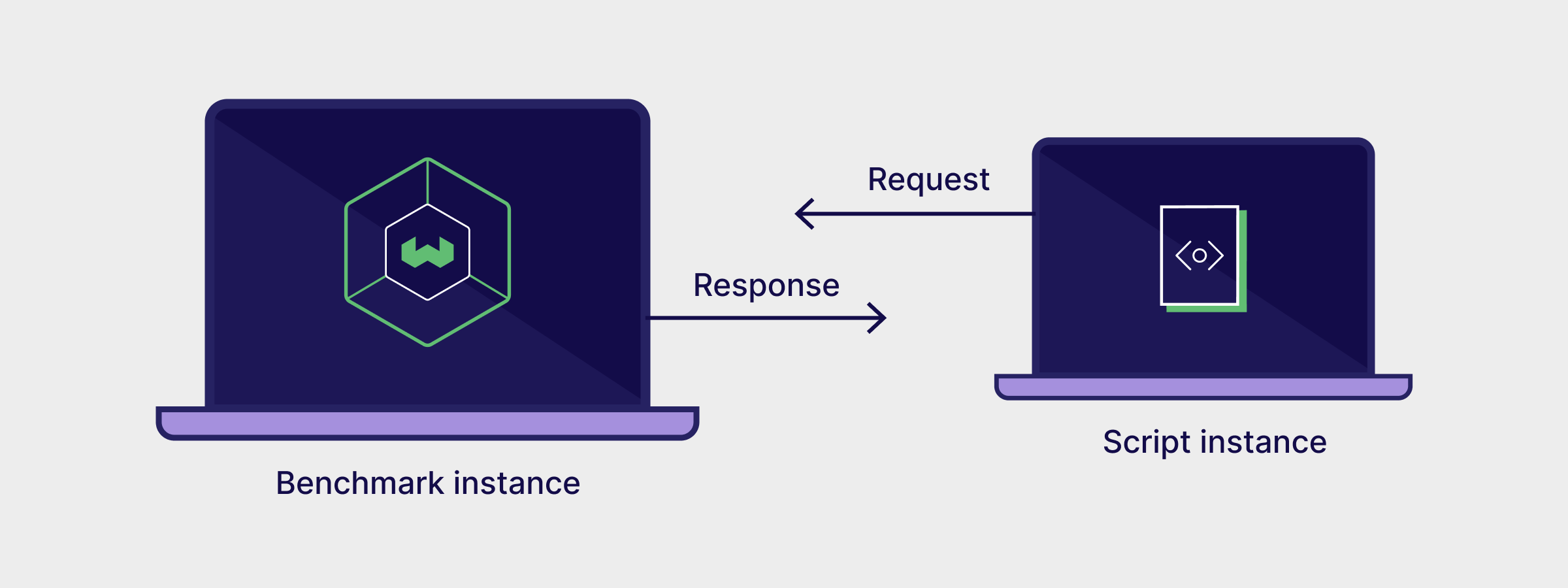
This benchmark test uses one GCP instances to run both Weaviate and the Benchmark scripts:

a n4-highmem-16 instance with 16 vCPU cores and 128 GB memory.

Based on your throughput requirements, it is very likely that you will run Weaviate on a considerably smaller or larger machine in production.

We have outlined in the Benchmark FAQs what you should expect when altering the configuration or setup parameters.

Experiment Setup

We modeled our dataset selection after ann-benchmarks. The same test queries are used to test speed, throughput, and recall. The provided ground truths are used to calculate the recall.

We use Weaviate's Golang client to import data. We use Go to measure the concurrent (multi-threaded) queries. Each language has its own performance characteristics. You may get different results if you use a different language to send your queries.

For maximum throughput, we recommend using the Go or Java client libraries.

The complete import and test scripts are available here.

Benchmark FAQ

How can I get the most performance for my use case?

If your use case is similar to one of the benchmark tests, use the recommended HNSW parameter configurations to start tuning.

For more instructions on how to tune your configuration for best performance, see HNSW Configuration Tips.

What is the difference between latency and throughput?

The latency refers to the time it takes to complete a single request. This is typically measured by taking a mean or percentile distribution of all requests. For example, a mean latency of 5ms means that a single request takes, on average, 5ms to complete. This does not say anything about how many queries can be answered in a given timeframe.

If Weaviate were single-threaded, the throughput per second would roughly equal to 1s divided by mean latency. For example, with a mean latency of 5ms, this would mean that 200 requests can be answered in a second.

However, in reality, you often don't have a single user sending one query after another. Instead, you have multiple users sending queries. This makes the querying side concurrent. Similarly, Weaviate can handle concurrent incoming requests. We can identify how many concurrent requests can be served by measuring the throughput.

We can take our single-thread calculation from before and multiply it with the number of server CPU cores. This will give us a rough estimate of what the server can handle concurrently. However, it would be best never to trust this calculation alone and continuously measure the actual throughput. This is because such scaling may not always be linear. For example, there may be synchronization mechanisms used to make concurrent access safe, such as locks. Not only do these mechanisms have a cost themselves, but if implemented incorrectly, they can also lead to congestion, which would further decrease the concurrent throughput. As a result, you cannot perform a single-threaded benchmark and extrapolate what the numbers would be like in a multi-threaded setting.

All throughput numbers ("QPS") outlined in this benchmark are actual multi-threaded measurements on a 30-core machine, not estimations.

What is a p99 latency?

The mean latency gives you an average value of all requests measured. This is a good indication of how long a user will have to wait on average for their request to be completed. Based on this mean value, you cannot make any promises to your users about wait times. 90 out of 100 users might see a considerably better time, but the remaining 10 might see a significantly worse time.

Percentile-based latencies are used to give a more precise indication. A 99th-percentile latency - or "p99 latency" for short - indicates the slowest request that 99% of requests experience. In other words, 99% of your users will experience a time equal to or better than the stated value. This is a much better guarantee than a mean value.

In production settings, requirements - as stated in support plans - are often a combination of throughput and a percentile latency. For example, the statement "3000 QPS at p95 latency of 20ms" conveys the following meaning.

3000 requests need to be successfully completed per second
95% of users must see a latency of 20ms or lower.
There is no assumption about the remaining 5% of users, implicitly tolerating that they will experience higher latencies than 20ms.

The higher the percentile (e.g. p99 over p95) the "safer" the quoted latency becomes. We have thus decided to use p99-latencies instead of p95-latencies in our measurements.

What happens if I run with fewer or more CPU cores than on the example test machine?

The benchmark outlines a QPS per core measurement. This can help you make a rough estimation of how the throughput would vary on smaller or larger machines. If you do not need the stated throughput, you can run with fewer CPU cores. If you need more throughput, you can run with more CPU cores.

Adding more CPUs reaches a point of diminishing returns because of synchronization mechanisms, disk, and memory bottlenecks. Beyond that point, you should scale horizontally instead of vertically. Horizontal scaling with replication is also available.

What are `ef`, `efConstruction`, and `maxConnections`?

These parameters refer to the HNSW build and query parameters. They represent a trade-off between recall, latency & throughput, index size, and memory consumption. This trade-off is highlighted in the benchmark results.

I can't match the same latencies/throughput in my own setup. How can I debug this?

If you are encountering other numbers in your own dataset, here are a couple of hints to look at:

What CPU architecture are you using? The benchmarks above were run on a GCP c2 CPU type, which is based on amd64 architecture. Weaviate also supports arm64 architecture, but not all optimizations are present. If your machine shows maximum CPU usage but you cannot achieve the same throughput, consider switching the CPU type to the one used in this benchmark.
Are you using an actual dataset or random vectors? HNSW is known to perform considerably worse with random vectors than with real-world datasets. This is due to the distribution of points in real-world datasets compared to randomly generated vectors. If you cannot achieve the performance (or recall) outlined above with random vectors, switch to an actual dataset.
Are your disks fast enough? While the ANN search itself is CPU-bound, the objects must be read from disk after the search has been completed. Weaviate uses memory-mapped files to speed this process up. However, if not enough memory is present or the operating system has allocated the cached pages elsewhere, a physical disk read needs to occur. If your disk is slow, it could then be that your benchmark is bottlenecked by those disks.
Are you using more than 2 million vectors? If yes, make sure to set the vector cache large enough for maximum performance.

Where can I find the scripts to run this benchmark myself?

The repository is located here.

Questions and feedback

Have a question or feedback? Here's how to reach us.

Community Forum

Ask questions and connect with other developers on our Community forum.

Support

Weaviate Cloud user or customer? Find the right channel on the Support page.

Measured Metrics

Benchmark Results

Benchmark Datasets

QPS vs Recall for DBPedia OpenAI

Recommended configuration for DBPedia OpenAI ada002

QPS vs Recall for SIFT1M

Recommended configuration for SIFT1M

QPS vs Recall for MSMARCO Snowflake

Recommended configuration for MSMARCO Snowflake

QPS vs Recall for Sphere DPR

Recommended configuration for Sphere DPR

Benchmark Setup

Scripts

Hardware

Experiment Setup

Benchmark FAQ

How can I get the most performance for my use case?

What is the difference between latency and throughput?

What is a p99 latency?

What happens if I run with fewer or more CPU cores than on the example test machine?

What are ef, efConstruction, and maxConnections?

I can't match the same latencies/throughput in my own setup. How can I debug this?

Where can I find the scripts to run this benchmark myself?

Questions and feedback

What are `ef`, `efConstruction`, and `maxConnections`?