Compression (Vector Quantization)
Vector quantization reduces the memory footprint of the vector index by compressing the vector embeddings, and thus reduces deployment costs and improves the speed of the vector similarity search process.
Weaviate currently offers four vector quantization techniques:
- Binary quantization (BQ)
- Product quantization (PQ)
- Scalar quantization (SQ)
- Rotational quantization (RQ)
What is quantization?
Section titled “What is quantization?”In general, quantization techniques reduce the memory footprint by representing numbers with lower precision numbers, like rounding a number to the nearest integer. In neural networks, quantization reduces the values of the weights or activations of the model stored as a 32-bit floating-point number (4 bytes) to a lower precision number, such as an 8-bit integer (1 byte).
What is vector quantization?
Section titled “What is vector quantization?”Vector quantization is a technique that reduces the memory footprint of vector embeddings. Vector embeddings have been typically represented as 32-bit floating-point numbers. Vector quantization techniques reduce the size of the vector embeddings by representing them as smaller numbers, such as 8-bit integers or binary numbers. Some quantization techniques also reduce the number of dimensions in the vector embeddings.
Product quantization
Section titled “Product quantization”Product quantization is a multi-step quantization technique that is available for use with hnsw indexes in Weaviate.
PQ reduces the size of each vector embedding in two steps. First, it reduces the number of vector dimensions to a smaller number of "segments", and then each segment is quantized to a smaller number of bits from the original number of bits (typically a 32-bit float).
PQ makes tradeoffs between recall, performance, and memory usage. This means a PQ configuration that reduces memory may also reduce recall. There are similar trade-offs when you use HNSW without PQ. If you use PQ compression, you should also tune HNSW so that they compliment each other.
In PQ, the original vector embedding is represented as a product of smaller vectors that are called 'segments' or 'subspaces.' Then, each segment is quantized independently to create a compressed vector embedding.
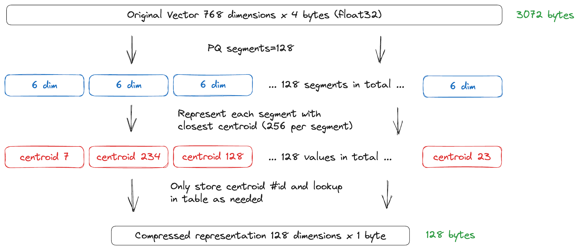
After the segments are created, there is a training step to calculate centroids for each segment. By default, Weaviate clusters each segment into 256 centroids. The centroids make up a codebook that Weaviate uses in later steps to compress the vector embeddings.
Once the codebook is ready, Weaviate uses the id of the closest centroid to compress each vector segment. The new vector embedding reduces memory consumption significantly. Imagine a collection where each vector embedding has 768 four byte elements. Before PQ compression, each vector embeddingrequires 768 x 4 = 3072 bytes of storage. After PQ compression, each vector requires 128 x 1 = 128 bytes of storage. The original representation is almost 24 times as large as the PQ compressed version. (It is not exactly 24x because there is a small amount of overhead for the codebook.)
To enable PQ compression, see Enable PQ compression
Segments
Section titled “Segments”The PQ segments controls the tradeoff between memory and recall. A larger segments parameter means higher memory usage and recall. An important thing to note is that the segments must divide evenly the original vector dimension.
Below is a list segment values for common vectorizer modules:
| Module | Model | Dimensions | Segments |
|---|---|---|---|
| openai | text-embedding-ada-002 | 1536 | 512, 384, 256, 192, 96 |
| cohere | multilingual-22-12 | 768 | 384, 256, 192, 96 |
| huggingface | sentence-transformers/all-MiniLM-L12-v2 | 384 | 192, 128, 96 |
PQ compression process
Section titled “PQ compression process”PQ has a training stage where it creates a codebook. We recommend using 10,000 to 100,000 records per shard to create the codebook. The training step can be triggered manually or automatically. See Configuration: Product quantization for more details.
When the training step is triggered, a background job converts the index to the compressed index. While the conversion is running, the index is read-only. Shard status returns to READY when the conversion finishes.
Weaviate uses a maximum of trainingLimit objects (per shard) for training, even if there are more objects available.
After the PQ conversion completes, query and write to the index as normal. Distances may be slightly different due to the effects of quantization.
Encoders
Section titled “Encoders”In the configuration above you can see that you can set the encoder object to specify how the codebook centroids are generated. Weaviate's PQ supports using two different encoders. The default is kmeans which maps to the traditional approach used for creating centroid.
Alternatively, there is also the tile encoder. This encoder is currently experimental but does have faster import times and better recall on datasets like SIFT and GIST. The tile encoder has an additional distribution parameter that controls what distribution to use when generating centroids. You can configure the encoder by setting type to tile or kmeans the encoder creates the codebook for product quantization. For configuration details, see Configuration: Vector index.
Distance calculation
Section titled “Distance calculation”With product quantization, distances are then calculated asymmetrically with a query vector with the goal being to keep all the original information in the query vector when calculating distances.
Binary quantization
Section titled “Binary quantization”Binary quantization (BQ) is a quantization technique that converts each vector embedding to a binary representation. The binary representation is much smaller than the original vector embedding. Usually each vector dimension requires 32 bits, but the binary representation only requires 1 bit, representing a 32x reduction in storage requirements. This works to speed up vector search by reducing the amount of data that needs to be read from disk, and simplifying the distance calculation.
The tradeoff is that BQ is lossy. The binary representation by nature omits a significant amount of information, and as a result the distance calculation is not as accurate as the original vector embedding.
Some vectorizers work better with BQ than others. Anecdotally, we have seen encouraging recall with Cohere's V3 models (e.g. embed-multilingual-v3.0 or embed-english-v3.0), and OpenAI's ada-002 model with BQ enabled. We advise you to test BQ with your own data and preferred vectorizer to determine if it is suitable for your use case.
Note that when BQ is enabled, a vector cache can be used to improve query performance. The vector cache is used to speed up queries by reducing the number of disk reads for the quantized vector embeddings. Note that it must be balanced with memory usage considerations, with each vector taking up n_dimensions bits.
Scalar quantization
Section titled “Scalar quantization”Scalar quantization (SQ) The dimensions in a vector embedding are usually represented as 32 bit floats. SQ transforms the float representation to an 8 bit integer. This is a 4x reduction in size.
SQ compression, like BQ, is a lossy compression technique. However, SQ has a much greater range. The SQ algorithm analyzes your data and distributes the dimension values into 256 buckets (8 bits).
SQ compressed vectors are more accurate than BQ compressed vectors. They are also significantly smaller than uncompressed vectors.
The bucket boundaries are derived by determining the minimum and maximum values in a training set, and uniformly distributing the values between the minimum and maximum into 256 buckets. The 8 bit integer is then used to represent the bucket number.
The size of the training set is configurable. The default is 100,000 objects per shard.
When SQ is enabled, Weaviate boosts recall by over-fetching compressed results. After Weaviate retrieves the compressed results, it compares the original, uncompressed vectors that correspond to the compressed result against the query. The second search is very fast because it only searches a small number of vectors rather than the whole database.
Rotational quantization
Section titled “Rotational quantization”Rotational quantization (RQ) provides significant compression while maintaining high recall. Unlike SQ, RQ requires no training phase and can be enabled immediately at index creation. RQ is available in: 8-bit, 4-bit and 1-bit variants.
8-bit RQ
Section titled “8-bit RQ”8-bit RQ provides 4x compression while maintaining 98-99% recall in internal testing. The method works as follows:
-
Fast pseudorandom rotation: The input vector is transformed using a fast rotation based on the Walsh Hadamard Transform. This rotation takes approximately 7-10 microseconds for a 1536-dimensional vector. The output dimension is rounded up to the nearest multiple of 64.
-
Scalar quantization: Each entry of the rotated vector is quantized to an 8-bit integer. The minimum and maximum values of each individual rotated vector define the quantization interval.
4-bit RQ
Section titled “4-bit RQ”4-bit RQ stores each dimension of the rotated vector in 4 bits, so a compressed vector is about half the size of the 8-bit equivalent and roughly 8x smaller than the uncompressed vector. It sits between 8-bit RQ and 1-bit RQ: it gives up some accuracy in the compressed distance calculation in exchange for a smaller index.
The method works as follows:
-
Fast pseudorandom rotation: The same rotation process as 8-bit RQ is applied to the input vector, and the output dimension is rounded up to the nearest multiple of 64. Because the output dimension is always a multiple of 64, two codes always pack cleanly into one byte.
-
Asymmetric quantization:
- Data vectors: Quantized to 4 bits per dimension, over the minimum and maximum values of each individual rotated vector. Two dimensions are packed into each stored byte.
- Query vectors: Scalar quantized using 8 bits per dimension during search.
Quantizing the query at a higher precision than the stored data costs no extra storage and recovers much of the accuracy that the coarser data codes give up. This is the same asymmetric idea used by 1-bit RQ.
Because the compressed distances are coarser, 4-bit RQ depends more heavily on rescoring than 8-bit RQ does. In internal testing on 1536-dimensional data, 4-bit RQ reaches around 94-95% recall from the compressed distances alone, compared with around 99% for 8-bit RQ. In the same tests, rescoring the top 50 candidates against the uncompressed vectors brought both variants to 99.8% or better. See Configuration: 4-bit RQ.
1-bit RQ
Section titled “1-bit RQ”1-bit RQ is an asymmetric quantization method that provides close to 32x compression as dimensionality increases. 1-bit RQ serves as a more robust and accurate alternative to BQ with only a slight performance trade-off (approximately 10% decrease in throughput in internal testing compared to BQ). While more performant than PQ in terms of encoding time and distance calculations, 1-bit RQ typically offers slightly lower recall than well-tuned PQ.
The method works as follows:
-
Fast pseudorandom rotation: The same rotation process as 8-bit RQ is applied to the input vector. For 1-bit RQ, the output dimension is always padded to at least 256 bits to improve performance on low-dimensional data.
-
Asymmetric quantization:
- Data vectors: Quantized using 1 bit per dimension by storing only the sign of each entry
- Query vectors: Scalar quantized using 5 bits per dimension during search
This asymmetric approach improves recall compared to symmetric 1-bit schemes (such as BQ) by using more precision for query vectors during distance calculation. On datasets well-suited for BQ (like OpenAI embeddings), 1-bit RQ essentially matches BQ recall. It also works well on datasets where BQ performs poorly (such as SIFT).
RQ characteristics
Section titled “RQ characteristics”The rotation step provides multiple benefits. It tends to reduce the quantization interval and decrease quantization error by distributing values more uniformly. It also distributes the distance information more evenly across all dimensions, providing a better starting point for distance estimation.
All RQ variants round up the number of dimensions to multiples of 64, which means that low-dimensional data (< 64 or 128 dimensions) might result in less than optimal compression. Additionally, several factors affect the actual compression rates:
- Auxiliary data storage: 16 bytes for 8-bit and 4-bit RQ and 8 bytes for 1-bit RQ are stored with the compressed codes
- Dimension rounding: Dimensionality is rounded up to the nearest multiple of 64 and 1-bit RQ is also padded to at least 256 bits
Due to these factors, the 4x, 8x and 32x compression rates are only approached as dimensionality increases. These effects are more pronounced for low-dimensional vectors.
While inspired by extended RaBitQ, this implementation differs significantly for performance reasons. It uses fast pseudorandom rotations instead of truly random rotations.
Over-fetching / re-scoring
Section titled “Over-fetching / re-scoring”Weaviate over-fetches results and then re-scores them when you use SQ, RQ, or BQ. This is because the distance calculation on the compressed vectors is not as accurate as the same calculation on the original vector embedding.
When you run a query, Weaviate compares the query limit against a configurable rescoreLimit parameter.
The query retrieves compressed objects until the object count reaches whichever limit is greater. Then, Weaviate fetches the original, uncompressed vector embeddings that correspond to the compressed vectors. The uncompressed vectors are used to recalculate the query distance scores.
For example, if a query is made with a limit of 10, and a rescore limit of 200, Weaviate fetches 200 objects. After rescoring, the query returns top 10 objects. This process offsets the loss in search quality (recall) that is caused by compression.
Vector compression with vector indexing
Section titled “Vector compression with vector indexing”With an HNSW index
Section titled “With an HNSW index”An HNSW index can be configured using PQ, SQ, RQ, or BQ. Since HNSW is in memory, compression can reduce your memory footprint or allow you to store more data in the same amount of memory.
If memory is your main constraint, you can also consider the disk-based HFresh index as an index-level alternative to compression: it keeps only a compressed centroid index in memory and stores the rest on disk.
With a flat index
Section titled “With a flat index”RQ and BQ can be applied to a flat index. As a flat index search is a brute-force method, compression reduces the amount of data Weaviate has to read and increases speed.
A flat index accepts 8-bit and 1-bit RQ. 4-bit RQ is available for the HNSW index only.
Rescoring
Section titled “Rescoring”Quantization inherently involves some loss information due to the reduction in information precision. To mitigate this, Weaviate uses a technique called rescoring, using the uncompressed vectors that are also stored alongside compressed vectors. Rescoring recalculates the distance between the original vectors of the returned candidates from the initial search. This ensures that the most accurate results are returned to the user.
In some cases, rescoring also includes over-fetching, whereby additional candidates are fetched to ensure that the top candidates are not omitted in the initial search.
Further resources
Section titled “Further resources”Questions and feedback
Section titled “Questions and feedback”Have a question or feedback? Here's how to reach us.